Structure from Motion (SfM) is a very useful tool for creating 3D models from unreferenced images. Since SfM can create highly detailed models from historic film and digital photographs, it is particularly helpful in examining changes in an object over time. In this short post I'll show how data collected at a pictograph site in 2003 can be compared with more recent data to pinpoint areas of deterioration in a systematic way.
The pictograph we'll be looking at is located at 41CX2 and is part of a prehistoric site on the eastern edge of the Pecos River in West Texas. I like to use data collected from this site because there are no issues with making it publically available. I also go back to it because there are both older digital photographs of the site and much older historic photographs archived at the Texas Archaeological Research Laboratory (TARL). This provides a nice test bed of data to take advantage of.
In order to compare a set of historic photographs with modern ones, aligning the two image sets to each other is critical. This can be difficult because photographs contain all sorts of lens distortions and it is hard to reproduce the exact angle of a historic photograph with a modern camera. It may sound like a simple task to overlay one image on another in Photoshop but getting an exact alignment between two photographs taken at different times, is almost impossible. SfM can aid in the alignment process. By analyzing the structure of the object in the photographs, SfM can remove virtually all distortion when a 3D model is created. Therefore, if you create one 3D model from historic photographs and another 3D model from more recent images, the two can almost perfectly aligned to each other. The easiest way to accomplish the alignment is by assigning the same coordinate system to each model and then converting those to a Digital Elevation Model (DEM).
2003 and 2011 SfM models aligned.
In this example, I have assigned the same arbitrary coordinate system to each model with the X and Y axis approximately in alignment with the natural surface of the rock. In other words, the Z, or elevation value, is greater the closer it is to the viewer and vice versa. With both models now in the same space and orientation, the Z values of the vertices can be sampled to create a DEM. It is important to note the word "sample" here because each cell of the DEM is composed of a value derived from the average value of the vertices that fall within that cell. If cell sizes are not the same or have a different origin point, the DEM values can vary slightly for what appears to be the same location. In our example the 2003 3D model covers a slightly larger area than that collected in 2011. Due to this difference in area, the DEM cells are slightly offset. To help reduce this minor alignment problem, the 2003 model could be clipped to the same size as the 2011 data but for this project I left the models in their original state.
2003 DEM
2011 DEM
The result of subtracting the 2011 DEM from the 2003 DEM.
Areas of red have had the greatest change.
Having created the DEMs for the 2003 and 2011 models, each DEM was loaded into ArcGIS. To compare the changes between the DEMs over time, the 2011 data was subtracted from the 2003 data. This was done with the Spatial Analyst's Raster Calculator tool. The resulting DEM highlights those areas of significant change in red and the more stable areas in blue. As mentioned previously, the DEM cell values do not match exactly so there is minor variation visible across the model. When the difference DEM is transposed against the pictograph images, areas of deterioration are obvious. While it is certainly possible to visually compare the photographs from different time periods and see that damage is taking place, this process allows for a systematic and quantifiable means of assessing that change.
2003 image imposed over differences map.
2011 image imposed over differences map.
Closeup of 2003 imagery and differences map.
Animation showing change from 2003 to 2011.
The implications for using this technique are exciting. Since SfM can work with historic film photographs, many older photographs of rock art panels can be analyzed and historic 3D models created. Furthermore, the process need not focus on pictographs; historic aerials can be converted to DEMs and geomorphological changes examined or the process could be applied to underwater photography to examine the morphological changes of coral reefs, etc. There are many possibilities.
A tutorial on hard copy printing of virtual models using 3DS Max and Shapeways
3D hard copy printout of pictograph.
There are now several rapid prototyping/3D printing services available for creating hard copy models of virtual creations. Here, I walk through the steps for preparing a Structure from Motion (SfM) model for color/textured printing using the services provided by Shapeways.com and 3D Studio Max 2009. Shapeways is an economical online service that accepts the upload of 3D files and then sends you a hard copy of that model you can hold in your hands.
Other than it just being plainly awesome, why create virtual models of rock art or other archaeological phenomena? Here are some reasons to consider:
Virtual models are easy to share with other researchers via the Internet. This may broaden interaction and scientific inquiry.
Public access to 3D models allows for remote or extremely delicate objects to be explored and enjoyed.
People love to touch archaeology. Holding a replica can fulfill some of this desire without damage to the real thing.
Elements that are not obvious in 2D may stand out in 3D, giving new insight about the object.
3D models create a virtual snapshot of an object in time that can be compared with future models to consider impacts and changes to the real object over time.
The 3D model can be modified so that certain aspects of it can be exaggerated. A good example would be the stretching a petroglyph model along its depth axis, making ridges taller and grooves deeper. Thus helping to show faint detail on the original.
Using emerging Structure from Motion (SfM) and photogrammetry techniques, highly accurate and detailed models can be created from historic photographs. This can allow for unique 3D views of lost elements or destroyed sites to be examined in new ways.
Creating a "water tight" 3D model in 3DS Max** **Please note, I am not an expert with 3D Studio Max. If anyone has a better way of doing anything described in this tutorial, please let me know.
Follow along with this tutorial on Youtube..
I start with the 3D model in Alias Wavefront OBJ format. The 3D was made from a series of photographs of a small prehistoric pictograph found in a rockshelter above the Pecos River in West Texas. The file consists of about 102,000 polygons and a texture in JPG format. 500,000 polygons is the largest number of polygons that Shapeways can currently handle. I purposefully created the model to have a little less than a half million polygons because additional structure will be added to the model.
The imported Alias Wavefront OBJ File in 3DS Max.
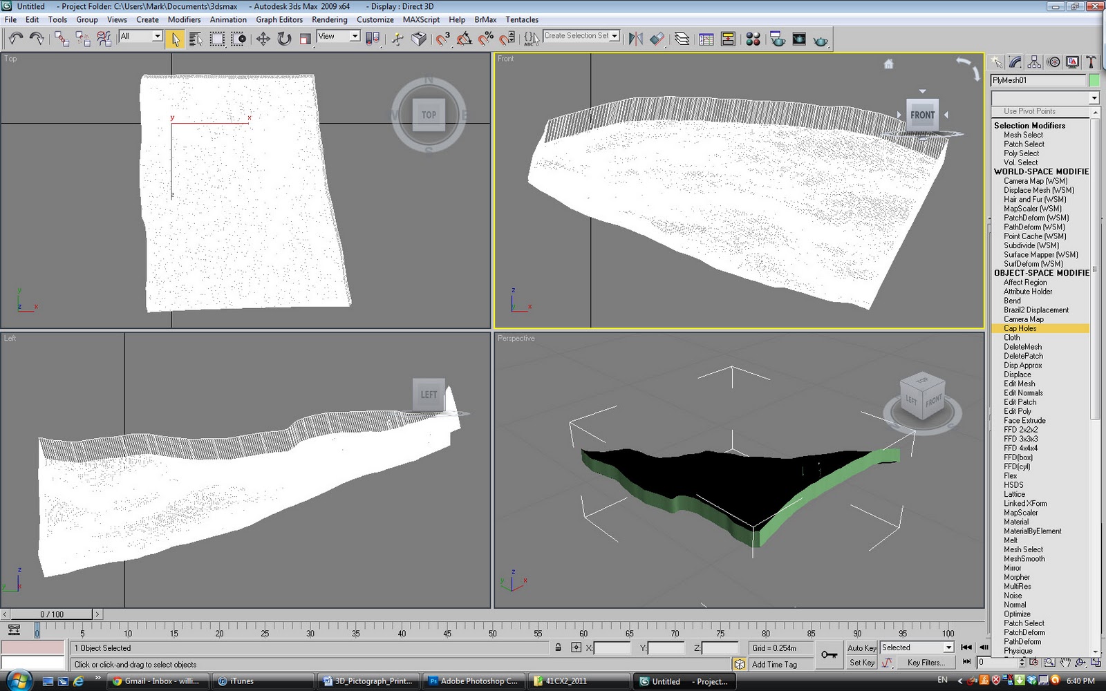
The first step is to import the OBJ file using Max's import command (File>Import). This particular 3D model is very flat and has no volume. Its shape is analogous to a slightly crumpled and twisted piece of paper. In order for the model to be printed, it must have volume and depth. It also has to be "watertight", lacking any holes or open faces. To give the model volume in Max, it is extruded by selecting it and then clicking the (Modify>Element) command and then selecting the entire model, and extruding it. In this example, it extruded it by a value of 0.004.
Extruding the edges of the model.
There are a few things to consider when the model is extruded. The model needs to be thick enough to be strong when printed but the thicker it is, the more it will cost to print. The hard copy price is calculated by volume and the material the object is printed from. The internal geometry of the model must be considered, too. With only the exterior edges of the model being extruded, enough of a buffer between the "bottom" of the model and extruded edge must be present or the model will be fragile or have holes.
Once the extrusion is just right, the model is converted to a mesh (right-click selected mesh>covert to editable mesh) and then a "Cap Holes" modifier is added (Modify>Cap Holes). This closes the "bottom" of the model and gives it volume. It is important at this stage to examine the model carefully and make sure nothing strange is going on with the geometry. To check this, I look at the model in wireframe mode and also render it (F10) from several vantage points. Certain faces may need to be adjusted (Modify>polygons>faces). The Cap Holes modifier is automatic and sometimes does not work very well. Be sure to check the model statistics to insure the model is still below 500,000 polygons. If it is not, the model needs to be decimated.
Converting the model to a mesh.
Adding the "Cap Holes" modifier.
Once satisfied the model will be strong, but thin enough to print affordably, the model is selected and exported as an STL file. The STL is then opened in netfabb Studio and tested. Netfabb is a free utility and details of its use are described in this tutorial. I use netfabb not only to identify problems, but actually fix the issues in Max. I do it this way because texture location is lost when the file is exported to STL. Luckily, most of the time, netfabb does not find any issues with the model.
To print the model in color a JPG, or similar texture map, is required. The resolution which Shapeways can print at is very limited in regards to the texture map. The maximum is 2048 x 2048 pixels; so, I resize the texture map in Photoshop and then apply that map in Max to and review it for proper alignment.
Applying the texture to the model.
Next, the 3D model needs to be scaled to the size it will be printed at. This can be a little tricky and can take some trial and error. I have found that scaling a model to about four meters in Max produces a hard copy printout about 15 cm in size.
Scaling the model up to "4 meters" in size.
Models that are to be printed with textures must be exported to VRML 2.0 (aka VRML97) format. In order to do this go to (File>Export>VRML). Check only "Indentation" in the Generate options section, leave Polygon Type as Triangles, set the Digits of Precision to 6, turn off the Bitmap URL Prefix radio button, and then click Ok. This will create a VRML formatted file with the suffix WRL. Next, compress the newly created VRML file along with texture map into a zip file. Make sure the zip file is less than 65 megabytes in size (it should be considerably smaller than that).
Exporting the textured 3D model to VRML97 format.
Upload the file to your Shapeways account. Set the upload units to millimeters and start the file transfer. An email should arrive from Shapeways saying that the file has arrived and later, another email describing if the model was viable or if there was a problem.
Uploading to Shapeways.
With a successful upload to Shapeways website, the size of the model can be checked and the cost of printing from different materials assessed. Keep in mind that only the "full color sandstone" option works with textured models. If the costs are too high or the model too small, recreate it at a different scale and re-upload. Once the model is the right size and price, place the order and it should arrive within a couple of weeks.
Picking the material to print the model in.
My model measures 10.2 w x 3.7 d x 14.3 h cm in size and cost $128.89, including shipping. The model appeared on my door step six days after it was uploaded. 3D printing is still in its infancy, especially for color, and the final model is not quite a perfect recreation. The baking/fusing process used made the colors slightly darker on the model than the original. The model also has contour-like shapes comprising its surface. This effect is caused by the laser that built up of the surface of the model, one layer at a time. Additionally, some of the rock edges are not as crisp as the real thing. Problems such as these are likely to go away as 3D printing evolves. All in all, the model gives a fairly accurate reproduction of the original surface of the rock and the pictograph's association with that surface.
3D printout.
Closeup photo of contour-like stair-stepping on the model's surface.
One thing I had not noticed when I visited the pictograph in person, was the slight protrusion of rock between the legs of the anthropomorph. Looking at the virtual model and hard copy, it becomes obvious that this element of the natural rock helped inform the artist's placement of the pictograph. Under closer examination, the rock directly above the protrusion appears to have been chipped away or modified in some other way. Does the protrusion represent genitalia? Could the chipped rock at the abdomen signify a pregnancy or mutilation? Having the 3D model to examine raises new questions that were not obvious to ask before its creation.
3D animation of pictograph at 41CX2.
The natural surface of the rock appears to have been an element
incorporated into the positioning of this pictograph.
I hope this tutorial was helpful and provided some insight into the usefulness of virtual recreations of rock art and other objects.
Introduction Here are initial results of a mapping exercise using a combination of inexpensive and innovative technologies. As part of a larger project, the mapping techniques were tested on a prehistoric burned rock midden (Feature 59). The feature, sometimes referred to as a ring midden by local archaeologists, measures about 18 meters in diameter and is more than one meter tall. It is just one out of more than a hundred burned rock features found at the Guadalupe Village Site in southern New Mexico.
Feature 59 in August 2010 after a very wet spring.
Feature 59 in July 2011 after wildfires hit the area.
We first aerially mapped the site in the summer of 2010 but had mixed results due to usually dense vegetation that had grown over it, following an uncommonly wet spring season. Wildfires burned much of that brush off in 2011 at which time my colleagues and I were invited back to the site for another go at it.
The focus of the main project was to document the site with Kite Aerial Photography (KAP) and Blimp Aerial Photography (BAP), though the data highlighted here were collected from a handheld pole. A makeshift Pole Aerial Photography (PAP) rig was cobbled together from a painter's telescoping pole, a modified paint roller, a "Tupperware" container, few zip-ties, and electrical tape. The rig allowed for a Canon A540 digital camera to be pointed straight down while suspended more than five meters above the ground. The camera was programmed to automatically take photographs every several seconds using the Canon Hackers Development Kit (CHDK) while running an intervalometer script.
Conducting PAP at Feature 59.
After clearing some of the burnt plants away from the feature, the PAP rig was slowly walked across the it in a series of transects. The objective was to take a number of overlapping photographs across the entire surface of the feature. 184 photos were collected in this fashion and, after setup, took less than an hour to complete.
Example of overlapping images collected during PAP.
Once back from the field, the number of photographs was culled by removing blurry and off-subject images. As a result, 158 photographs were processed using Structure from Motion (SfM) techniques and a textured high resolution 3D model was created.
Recently, I tested Polynomial Texture Mapping (PTM), a type of Reflection Transformation Imaging (RTI), to enhance petroglyphs in West Texas. I wondered if the same process could be applied, in a virtual sense, to the 3D model of the feature. To over-simplify it a bit, the PTM process involves taking a series of photographs (normally under dark conditions), while an off-camera flash is moved around the subject matter from set distances and angles. The images are then imported into a piece of software that allows the object to be examined as a polynomial representation of all the photographs combined. PTM often reveals details that are not visible to the naked eye and can even brings out structural elements not visible with laser scanning. Using this technique we are able to look at the form of the Feature 59 in a new way.
Creating the VPTM Model
Virtual lighting and camera setup in 3dsMax.
Virtual PTM renderings.
PTM of 3D model in PTMviewer software.
To create the PTM model, a set of virtual lights were positioned around the 3D model in 3D Studio Max. A total of 144 lights were stationed in dome-like fashion around the feature. A virtual glossy sphere was also created and placed next to feature. The sphere is used by the PTM building software as a reference for the location of each light source. Using this virtual photography studio, 144 images were rendered, one for each of the lighting locations. Finally, those images were fed into the PTMbuilder application through a java interface called LPTracker and a PTM file was created.
PTM rendering with possible sub-features highlighted.
The Virtual PTM (VPTM) reveals many aspects of the feature that are not visible in the textured model. It suggests that sub-features may have been excavated into the main feature or, at least that burned rock was removed from it at several places. Some of the possible sub-features are obvious when standing in front of the actual feature but, not all.
Generating a PTM is this fashion is particularly innovative because it would be almost impossible to do with the real life feature. Two cranes, one for the camera and another to move around a giant light, would have been needed to create a PTM of Feature 59 using the traditional approach. The use of VPTM on objects that do not allow for the systematic photography that a normal PTM requires, may reveal aspects that are impossible to see otherwise. Using VTPM with aerial photography is just one possibility. For example, the same process could be used on hard to reach rock art sites or within submerged caves.
Creating a VPTM from a 3D model has some pitfalls in that the VPTM can only be as good as the 3D model it is generated from. Any distortions in the 3D model that are an artifact of the SfM process could appear as prehistoric anomalies in the rendering. Researchers should consider this when making and evaluating similar models.
The feature documented here, used equipment that cost well under $250 (most of that for the camera). The PTM generating software is free. While the other software used is more expensive, free open source solutions capable of the same results are available. Considering the minor amount of time needed to collect the data, the low cost of the process, and the high quality results, other archaeologists should consider applying these techniques to sites anywhere they work.
Digital Elevation Model (DEM) of feature with 5 cm contours. Note that west is up.
Acknowledgments The initial work at the Guadalupe Village Site (LA 143472) was funded by a small Permian Basin MOA Grant through the Bureau of Land Management office in Carlsbad, New Mexico. The second visit to the site (which yielded this data) was done entirely pro bono. Archaeologists Juan Arias, Bruce Boeke, Tim Graves, Jeremy Iliff, and Myles Miller III made the project possible.