How to create a Digital Elevation Model from Photosynth point clouds

Recent developments in the Open Source community have made it easier to create 3D models from point cloud data derived from Structure from Motion (SfM) technologies such as Photosynth and Bundler.  This article outlines the steps I use to create Digital Elevation Models (DEM) from data acquired from kite, blimp, and UAV aerial photography.

In order to standardize this tutorial, I've created a set of data that you can follow along with using a Windows based computer.  All of the concepts described here should also work in a Linux environment with little modification. Useable examples of all the files created during this tutorial are available for download at www.palentier.com/DEM_Tutorial .

The point cloud used in this tutorial was created by me and is located on the Photosynth website at http://www.photosynth.net/view.aspx?cid=14d8887c-7475-42d5-b810-c6642eace2c5 .  The photographs that make up the synth were acquired from Kite Aerial Photography (KAP) and are of archaeological excavations at a pre-Inka tola site near the village of Palmitopamba in Ecuador.

I have attempted to use as many free and open source applications as possible but the final steps are completed in the commercial ArcGIS software. ArcGIS is the most widely used GIS program in the world and most users will probably be familiar with it.

The software needed for this tutorial are:

• Photosynth (which requires Silverlight)
• Photosynth Exporter
• Meshlab
• Excel or Open Office
• Notepad (built into Windows)
• ScanView
• Java Graticule 3D (JAG3D)
• ArcGIS with Spatial or 3D Analyst

Step 1

Place Ground Control Points (GCPs) around your subject matter in an evenly spaced pattern.  (I tend to use cheap paper plates as targets but if a point cloud is going to be processed in SfM software, it is best if the GCPs contrast starkly with the background).  The more GCPs that are placed the better.

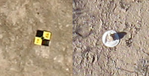Two examples of GCPs. The one on the left is a retroreflective target
and the one on the right is a paper plate with a rock on it.

Step 2

Take aerial photographs of the project area.  The photographs need to be taken high enough from the ground to view the GCPs, but low enough that resolution is not lost.  The higher you fly, the lower the resolution of the ground.  The lower you fly the more photographs and GCPs are needed.  It is a balancing act.  It is normally best to take photographs from various heights to insure proper coverage.  I normally take three to four thousand photographs - and review the images periodically during the process.

Taking aerial photographs of the site with a KAP rig.

A few of the aerial photographs taken from the kite.

Step 3

Record the location of each GCP.  Ideally, this is done with a Total Data Station (TDS).  A TDS will record highly accurate X, Y, and Z coordinates for each GCP. An alternative method is to use a GPS with a barometric altimeter.  I have tested an inexpensive Garmin Map 60Cx with this process and it works reasonably well, but the accuracy suffers.  Whichever method is used, save the coordinates to text file with the name "RealWorldGCPs.txt".

Recording the locations of the GCPs with the TDS.

Note: This method has only been tested with metric coordinates (ie. UTM) but it should work also work with data in decimal degrees.

Step 4

The next task is to cull the images.  Removing blurry and off-subject photographs is especially important when the photos come from blimp aerial photography (BAP) or kite aerial photography (KAP). Try to have 400 to 600 highly overlapping ‘in focus’ photographs of your subject matter.  Do not edit the photographs. Editing the photographs can cause problems in the next step.

Step 5

Process the photographs with Photosynth or Bundler.  This involves uploading your images to Photosynth or through the stand alone Bundler SfM application. 

Step 6

Review the point cloud data.  The creation of the point clouds often hits a snag and produces bad data.  To view the point cloud in Photosynth, press the "P" on your keyboard a couple of times while viewing the synth.  This will step through showing photographs and point clouds.  If your project has a low synth value or has a large amount of points in places they should not be, reprocessing of the data is needed.  Try adding or removing photographs to improve the model.  This involves re-uploading and reprocessing your images. Ideally, the project will be “100% Synthy” on Photosynth’s “Synthy” scale but 100% “synthiness” is not mandatory to get good results.

The point cloud as viewed in Photosynth.

Step 7

Extract the point cloud. If using Photosynth, the free Photosynth Exporter application can extract the data.  In Photosynth Exporter, select "From URL" and then paste the synth URL into the open field.  To follow along with my data use the URL " http://www.photosynth.net/view.aspx?cid=14d8887c-7475-42d5-b810-c6642eace2c5 ". Make sure PLY (ASCII) (not binary) is selected.  A new dialog box will open, from "Select point clouds to export" choose the default option of "0*" and then click "Ok". Name it "Tola_5_0.ply". If denser point clouds are needed, use Photosynth’s Tool Kit.  Either process will produce a PLY model of the point cloud.

Download the point cloud with Photosynth Exporter.

Step 8

Open the file "Tola_5_0.ply" and edit the point cloud using the free and open source Meshlab software.  It is likely that some stray points or noise exist in the point cloud and need to be removed.  Use Meshlab's "Select Vertexes" and "Delete the current set of selected vertices" tools to accomplish this. 

Editing the point cloud in Meshlab.

Step 9

Save the edited point cloud with the name "Tola_5_0_edited.ply" again - make sure it is an ASCII (not binary) formatted PLY.

Saving the edited point cloud as an ASCII file in Meshlab.

Step 10

Open the newly edited point cloud file "Tola_5_0_edited.ply" in a text editor like Notepad and delete the header. 

The part you want to delete will look similar to this:

plyformat ascii 1.0comment VCGLIB generatedelement vertex 134399property float xproperty float yproperty float zproperty uchar redproperty uchar greenproperty uchar blueproperty uchar alphaelement face 0property list uchar int vertex_indicesend_header

This will leave only the set of X, Y, and Z attributes.  Save the file with the name "pointcloud_edited.XYZ". This file will be used later in the tutorial.

Removing the header from Tola_5_0_edited.ply.

The edited file ready to save as pointcloud_edited.XYZ.

Step 11

Next open "Tola_5_0.ply"  from Step 8 (Not "Tola_5_0_edited.ply") in Notepad and delete the header.

The part you want to delete will look similar to this:

ply

format ascii 1.0

element vertex 137808

property float x

property float y

property float z

property uchar red

property uchar green

property uchar blue

end_header

This will leave only the set of X, Y, and Z attributes.  Save the file with the name "pointcloud_UNedited.XYZ". This file will be used later in the tutorial.

Removing the header from Tola_5_0.ply.

The file ready to be saved as pointcloud_UNedited.XYZ.

Step 12

The next several steps were developed by Nathan Craig and are also outlined on his blog.  They are recreated here with his permission. Note that my method does not maintain the point cloud vertex color as it is not needed/used in DEM creation.

ScanView is a free program to view and mark points within a point cloud.  You can use the import command to open the "pointcloud_UNedited.XYZ"  file saved in Step 11.  Use Scanview to locate the GCPs in the point cloud. Often it will be impossible to relocate all the GCPs in more sparse point clouds.  Focus on finding four or more widely distributed GCPs, if possible.  As GCPs are located, use the measure tool to record the location of each by pressing SHIFT and Left Clicking.  It is useful to write down which Scanview point cloud GCP number corresponds to the physical GCP numbers created in Step 3.  In other words, the GCP that was placed in the field may be GCP 12 but it corresponds to point cloud location 3 as recorded in Scanview.  I find it useful to have a printout of the GCPs real locations on a Google Earth background for reference and to use field notes.

Marking GCPs in ScanView.

Map used for reference.

Step 13

Once finished with identifying the point cloud GCPs, click the copy button in the measure tool.  This saves the data to the computer's virtual clipboard.  Open Notepad and paste this data into an empty file.

This will produce a tab delimited array according to the following format:

ID X Y Z

ID = the ScanView's point cloud GCP number.

XYZ = the point cloud location for each GCP.  These will often be values less than “10" and greater than “-10”.

Save this file as PointCloudGCPs.txt

Copying the points from ScanView to Notepad.

Step 14

Open Excel or similar spreadsheet program. Excel 2010 is capable of handling more than a million rows of data.  Older versions of Excel and all versions of Open Office can only handle about 65,000 rows of data.  This is important to note because most high resolution point clouds will have hundreds of thousands of points.

In Excel, go to Open and then choose the file type as "Text Files". Navigate to the location of the file PointCloud_edited.XYZ from Step 10.  In the filename box, type "*.XYZ" to make the file visible to Excel and then double click on the PointCloud_edited.XYZ file to open it.  A Text Import Wizard will pop up. Make sure the radio button for Delimited is selected and then click Next.  Depending on how the data was saved, you'll either need to select the "Space" or "Tab" boxes to properly delimit the file.  You will know you have it right when six vertical lines appear in the data preview box that divides the data into seven columns.  Click Finish and six columns of numbers should appear in the spread sheet.  The columns are in the format of X Y Z R G B 255.  The “XYZ” being the point cloud location of each point and “RGB” is the color value for each point.

Importing PointCloud_edited.XYZ into Excel.

The file PointCloud_edited.XYZ after import into Excel.

Step 15

The columns must be rearranged and modified for use in later steps.  In the Excel spread sheet, add a new column to the left of XYZ and delete the RGB and 255 columns.  This will leave the data in following format:

B X Y Z B B B B

B = BLANK/Empty column

PointCloud_edited.XYZ with unneeded columns removed and reorganized



Please note this process ignores the RGB values because they are not significant for the final DEM.  If you plan on using the data in 3D Studio Max or similar program, it may be useful to maintain these values.  See Nathan Craig's blog for more information on this.

Step 16

Open the file PointCloudGCPs.txt in Notepad. Select all the points and paste them into first rows of the PointCloud_edited.XYZ file opened in Excel.  This will replace several rows of data at the top of the file.  You may need to manually reformat this file in Notepad to get it to paste correctly.  Now select the first B column and use Excel's FILL command to add a series of numbers for each of the rows in the file.  This should start with 0 and end with whatever number aligns with your last row of data.  For each of the other columns, fill the rows with a value of 0. It should look something like this:

Step 17

Now select all the data in the Excel file and press CTRL-C to copy the data to the clipboard.  Next, open a new Notepad document and paste (CTRL-V) the data into it.  Save this file as "PointCloud_proc.txt" and close it.  Also save the Excel data as a backup before closing the program, in case a problem is encountered.

PointCloud_proc.txt

Step 18

Now open the "RealWorldGCPs.txt" file that was created in Step 3.  This file contains the real world locations of the GCPs but must be reformatted so that data in each row corresponds to each row of data in PointCloudGCPs.txt.  This may mean that rows need to be switched, renumbered, and removed.  Use notes and other reference materials noted in Step 12 to help with this task. Save the new file as "RealWorldGCPs_Reformatted.txt".

Matching the GCPs in RealWorldGCPs.txt to corresponds
to each available point in PointCloudGCPs.txt.

Step 19

The data is now properly formatted for use in the open source Java Graticule 3D (JAG3D) program. JAG3D transforms the arbitrary synth coordinate system into a real world coordinate system.   The commands for transforming the data are only available in German.  Open the program by double clicking the JAG3D.exe icon, click Module, and then choose Coordinate transformation (German only).  This will open a new window.  Make sure the 3D radio button is selected.  Next pick the 9-Parametertranformation-3D (Mx, My, Mz, Rx, Ry, Rz, Tx, Ty, Tz) from the drop down menu.  Now click Datei in the upper left of the menu and then Import Startsystem.  Next, pick the file "PointCloud_proc.txt" that was saved in Step 17.  This may take a while to open.  Once it has opened, click Datei again and then Import Zeilsystem. Now pick the file "RealWorldGCPs_Reformatted.txt" that was created in Step 18. To perform the transformation, click the "Berechnung starten" button in the lower right of the CoordTrans window.  This may take several minutes to complete.

PointCloud_proc.txt loaded into JAG3D.

RealWorldGCPs_Reformatted.txt loaded into JAG3D.

Step 20

To export the transformed coordinate file, click Datei in the upper left of the window and then Export Transformation.  Save this file with the name PointCloudinRealWorldCoordinates_trans.txt.

The data is now properly formatted, transformed, and is ready to be converted into a DEM.  The process for doing this in ArcGIS via the Spatial Analyst tool is explained here, but there are different software options available that are capable of this such as Golden Software's Surfer, ERDAS Image, or the open source GRASS software.

Step 21

The file PointCloudinRealWorldCoordinates_trans.txt must be imported into Excel.  The easiest way to do this is to open a new workbook in Excel.  Next, open PointCloudinRealWorldCoordinates_trans.txt in Notepad.  Select all the data (CTRL-A) and copy it to the clipboard (CTRL-C).  Now click the first column and row in Excel and paste the data (CTRL-V).  To create a header that ArcGIS can read, name the first column "Number", the second column "Easting", the third "Northing", the fourth "Elevation" and the final three columns A, B, and C.  Save this file in Excel's native format PointCloudinRealWorldCoordinates_trans.XLSX.

Bringing the JAG3D transformed output back into Excel.

Step 22

Open ArcGIS. We will need to create a shapefile from the transformed point cloud data using the Add XY Data tool.  Go to the main tool bar select Tools > Add XY Data.  Now navigate to the file saved in Step 21 (PointCloudinRealWorldCoordinates_trans.XLSX) from the "Choose a table from the map or browse for another table:" drop down.  Pick "Sheet 1" and click Ok. For the X Field choose the Easting (X) column. From the Y Field pick the Northing (Y) column.  Next define the coordinate system by choosing Edit from the lower left. The tutorial data is in the UTM Zone 17 North PSAD 56 projection. This will create an entry under Layers called "Sheet1$ Events" or something similar.  Right click on this file and choose Data > Export Data.  A warning "Table does not have Object_ID field" will appear. Click "Ok".  It will ask for an Output shapefile or feature class.  Call it "PointCloudinRealWorldCoordinates_trans.shp" and click OK. ArcGIS will ask if you would like to add the new shapefile as a layer.  Click yes. A new shapefile called PointCloudinRealWorldCoordinates_trans should appear in the layers display.  To keep this from becoming confusing, remove "Sheet1$ Events" by right clicking it and choosing "Remove".

Importing the transformed point cloud from Excel into ArcGIS.

Converting the Excel data into a shapefile.

Step 23

ArcGIS is not good at dealing with irregularly shaped point clouds during the DEM creation process. In order to make the dataset more ArcGIS friendly, the dataset must be rectangular.  To accomplish this, use the "Editor" drop down and then select "Start editing".  Next make sure the "Edit Tool" is active (It is the little black triangle next Editor drop down).  Now select a rectangular or square area that is entirely contained within the "PointCloudinRealWorldCoordinates_Trans" shapefile. Right click on "PointCloudinRealWorldCoordinates_trans" in the Layers window and then select "Open attribute table".  This will open a spread sheet of attributes for the shapefile.  Pick "Options" from the lower right of the spread sheet and then click "Switch Selection".  A warning may appear that says "This table (potentially) contains a large number of records... Do you want to continue?".  Click Yes and the data outside of your original selection will become active. Now click "Delete" from your keyboard to remove these outside points.  A rectangle of points should be left. Close the "Attributes of PointCloudinRealWorldCoordiantes_trans" by clicking the X in the upper right corner of that window. Save the edits by clicking the Editor drop down and then choosing "Stop Editing".  A window will open asking if you want to save the edits.  Pick Yes.

Selecting a rectangular area to become a DEM from the irregular shapefile.

Inverting the selection and deleting the points outside of the rectangular area.

The remaining points to create the DEM with.

Step 24

Now, make sure that the Spatial Analyst tool is visible in ArcGIS.  If it is not, from the main tool bar select Tools > Customize and then put a checkmark next to "Spatial Analyst" and then click Close.  Now in the Spatial Analyst tool bar choose "Interpolate to Raster and then Kriging". This will open the Kriging dialog box.  For Input points: choose the shapefile "PointCloudinRealWorldCoordinates_trans.shp".  For Z value field: pick the Elevation or Z column.  Adjust the output cell size to value that is appropriate for your data.  It is often best to leave this at default at first. Everything else should be ok to leave as is. Click Ok.  A new file "Krige of PointCloudinRealWorldCoordinates_trans" should appear after a few minutes.  This is your DEM! 

Using Spatial Analyst to create temporary DEM.

Step 25

To save the DEM, right click "Krige of PointCloudinRealWorldCoordinates_trans" and pick Data > Export Data.  A dialog box will open.  Name the file "DEM_PointCloudingRealWorldCoordinates_trans.img" and use the IMG format and click Save.

There are many things that can affect the quality of a DEM. The point cloud data used in this tutorial was collected on a windy day from a kite aerial photography rig.  Much of the ground vegetation was moderately tall grasses and small shrubs.  Since it was windy, the vegetation was constantly swaying and changing position slightly.  This produces “noise” during the synth matching process.  Furthermore, near the excavations there were several poles, an excavation screening tripod, and a tarp protruding above the ground surface.  These points have created "spikes" in the DEM.  The spikes could have been minimized by more aggressive editing during Step 8.

The DEM

Step 26

Have a cold beer.  You deserve it! Maybe you'd like to buy me one?  Click the donate button at the top right of this page!

Optional Steps

Step 27 - Create Contours

To create topographic contours of the DEM, go to Spatial Analyst drop down and pick Surface Analysis and then Contour. A dialog box will open.  From there choose "Input surface" as DEM_Point_CloudinRealWorldCoordiantes_trans.img" and then pick a Contour interval of 0.5 meters. Under Output Features save the file as "Tola_5_50cm_Contours.shp" and click Ok.

Generating topographic contours in Spatial Analyst.

50 centimeter contours on DEM.

 Step 28 - Georeference Aerial Photograph

The Georeferencing tool is made available by clicking Tools from the main menu, then Customize, putting a checkmark next to "Georeferencing", and clicking Close. Add an aerial photograph that covers a lot of the project area by clicking "Add Data" and picking "IMG_4197.JPG" (available from www.palentier.com/DEM_Tutorial/ ). A warning about Unknown Spatial Reference will appear.  Click Ok to proceed and add the image to the Layers window. Add the shapefile "Tola_5_TDS_UTM_Points" from www.palentier.com/DEM_Tutorial to the Layer's window as well. In the Georeferencing tool, make sure the Layer dropdown has "IMG_4197.JPG" active and then click the "Add Control Points" tool (The icon looks like a green x with a line drawn to a red x). Match the GCP plates on the JPG to the points in the Tola_5_TDS_UTM_Points shapefile.  The aerial image will start to line up with the portions of the DEM.  As the image was not taken perfectly nadir and contains lens distortions, it is impossible to completely align all the GCP plates with the shapefile points.  Line it up as best as possible, knowing that distortion is present.  Removal of the distortion is a subject for another tutorial...  Once you are satisfied with alignment, click Georeferencing, then click rectify, name it "IMG_4197_Rectified.img" and save the new image.  The original IMG_4197.jpg can now be removed from the Layers windows and the new IMG_4197_Rectified.img can be added.  Double click the "IMG_4197_Rectified.img" file from the Layers window.  The Layers Properties dialog box will open.  Select the Symbology tab and place a check mark next to "Display Background Value (R, G, B), under Stretch Type choose "Minimum-Maximum", and then click Ok. There should now be a georeferenced aerial image above the DEM.

Georeferencing the aerial photograph.

Removing black background and fixing colors.

Properly aligned aerial with DEM and contours.

An example of the results of this process, when exported to Google Earth, is available here:  http://www.palentier.com/DEM_Tutorial/Tola_5_DEM_and_Aerial.kmz

Step 29 - Visualing the Data in 3D

Use ArcScene to visualize your data as seen in this Youtube video:

Notes:

• If your dataset is very large, you might want to break it into several smaller sets.  I have found that point clouds of around 100,000 points process happily in JAG3D.  Larger point clouds (1 million+ points) can take forever to transform or may crash. Breaking the point clouds into smaller batches is also a good way to get around the 65,000 column limit in older version of Excel or in Open Office.  To do this break the points from Step 10 into several smaller groups of points AFTER completing Step 13 and then follow the rest of the tutorial for each group of points through Step 20.  The same PointCloudGCPs.txt file can be used for each group of points during the JAG3D transformation process. After all the groups of points have been transformed, copy and paste the contents of each group into one large text file (just add one group at the end of the next) and then proceed with the rest of the tutorial.
• Consider the output number of digits in your transformed data.  Some software, like 3DS Max and Meshlab, will not properly handle numbers with lots of digits.  You may need to remove several leading digits (as explained here) to make your data render properly.
• If any of your GCPs were not identifiable in the point cloud but their location is within the boundary of the DEM, you can double check the DEM accuracy by comparing the GCP's Z value with the DEM's Z value.

Useful Links:

Nathan Craig's Blog posts:

http://www.personal.psu.edu/nmc15/blogs/anthspace/2010/02/structure-from-motion-point-clouds-to-real-world-coordinates.html

http://www.personal.psu.edu/nmc15/blogs/anthspace/2010/06/coordinate-shift-for-improved-3d-rendering-of-models-that-are-in-utm-coordinates.html

Josh Harle's Tutorials:

http://vimeo.com/user3453059